Analyzing Incidence and Prevalence Rates in Epidemiologic Data

Prevalence: The fraction of a population with a particular condition

The prevalence of a condition in a population is the proportion of the population that has that condition at any given moment. It’s calculated by creating a fraction with a numerator and a denominator. The denominator is the total population eligible to have the condition. The numerator is the number of individuals from the population who have the condition at a given time. If you divide this numerator by this denominator, you will calculate the prevalence of the condition in that population.

Prevalence can be expressed as a decimal fraction, a percentage, or a rate per so many (usually per 1,000, per 10,000, or per 100,000). For example, a 2021 survey found that 11.6 percent of the U.S. adult population has Type II diabetes. But a rarer outcome — such as a monthly hospitalization rate for those suffering from influenza — may be expressed as 31.7 per 100,000. The prevalence is expressed as the result of a calculation from this fraction, but stated as a rate so that it is easy to envision. It would be hard to envision that 0.0317 percent of influenza sufferers were hospitalized in one month. On the other hand, it is much easier to envision almost 32 people from a town with a population of 100,000 being hospitalized in one month — provided you also envision that everyone in the town had influenza.

Because prevalence is a proportion, it’s analyzed in exactly the same way as any other proportion. The standard error (SE) of a prevalence ratio can be estimated by the formula in Chapter 13. Confidence intervals (CIs) for a prevalence estimate can be obtained from exact methods based on the binomial distribution or from formulas based on the normal approximation to the binomial distribution. Also, prevalence can be compared between two or more populations using the chi-square or Fisher Exact test. For this reason, the remainder of this chapter focuses on how to analyze incidence rates.

Incidence: Counting new cases

The incidence of a condition is the rate at which new cases of that condition appear in a population. Incidence is generally expressed as an incidence rate (R), which — like prevalence — is a fraction. The numerator for incidence is defined as the number of observed events (N) in a particular time period. (Consider an event to mean that a member of the population goes from not having the condition to having the condition.) Take note that while incidence expresses the number of new cases of the condition in the numerator, in contrast, prevalence includes all cases — both new and existing — in the numerator. The denominator for incidence is defined as the number of individuals in the population who could have had the event multiplied by the interval of time being used. This is also called time exposed or exposure (E). So, the equation for incidence is the number of observed events divided by the exposure, which is (E): R = N/E.

Exposure is measured in units of person-time, such as person-days or person-years. Incidence rates are expressed as the number of cases per unit of person-time. The unit of person-time is used so that the incidence rate can at least be the size of a whole number so it is easier to interpret and compare.

The incidence rate should be estimated by counting events over a narrow enough interval of time so that the number of observed events is a small fraction of the total population studied. One year is narrow enough for calculating incidence of Type II diabetes in adults because 0.02 percent of the adult population develops diabetes in a year. However, one year isn’t narrow enough to be useful when considering the incidence of an acute condition like influenza. In influenza and other infectious diseases, the intervals of interest would be in terms of daily, weekly, and monthly trends. It’s not very helpful to know that 30 percent of the population came down with influenza in a one-year period.

Consider City XYZ, which has a population of 300,000 adults. None of them has been diagnosed with Type II diabetes. Suppose that in 2023, 30 adults from City XYZ were newly diagnosed with Type II diabetes. The incidence of adult Type II diabetes in City XYZ would be calculated with a numerator of 30 cases and a denominator of 300,000 adults in one year. Using the incidence formula, this works out to 0.0001 new cases per person-year. As described before, in epidemiology, rates are reconfigured to have at least whole numbers so that they are easier to interpret and envision. For this example, you could express City XYZ’s 2023 adult Type II diabetes incidence rate as 1 new case per 10,000 person-years, or as 10 new cases per 100,000 person-years.

Now imagine another city — City ABC — has a population of 80,0000 adults, and like with City XYZ, none of them had ever been diagnosed with Type II diabetes. Now, assume that in 2023, 24 adults from City ABC were newly diagnosed with Type II diabetes. City ABC’s 2023 incidence rate would be calculated as 24 cases in 80,000 individuals in one year, which works out to or 0.0003 new cases per person-year. To make the estimate comparable to City XYZ’s estimate, let’s express City ABC’s estimate as 30 new cases per 100,000 person-years. So, the 2023 adult Type II diabetes incidence rate in City ABC — which is 30 new cases per 100,000 person-years — is three times as large as the 2023 adult Type II diabetes incidence rate for City XYZ, which is 10 new cases for 100,000 person-years. (Looks like City ABC’s public health department needs to get advice from City XYZ!)

Understanding how incidence and prevalence are related

From the definitions and examples in the preceding sections, you see that incidence and prevalence are two related but distinct concepts. The incidence rate tells you how fast new cases of some condition arise in a population, and prevalence tells you what fraction of the population has that condition at any moment.

You may expect that conditions with higher incidence rates would have higher prevalence than conditions with lower incidence rates. This is true with common chronic conditions, such as hypertension. But if a condition is acute — including infectious diseases, such as influenza and COVID-19 — the duration of the condition may be short. In such a scenario, a high incidence rate may not be paired with a high prevalence. Relatively rare chronic diseases of long duration — such as dementia — have low yearly incidence rates, but as human health improves and humans live longer on average, the prevalence of dementia increases.

Expressing the precision of an incidence rate

The precision of an incidence rate (R) is expressed using a confidence interval (CI). The SE of R typically is not reported, because the event rate usually isn’t normally distributed. The SE is computed only as part of the CI calculation.

Random fluctuations in R are attributed entirely to fluctuations in the event count (N). We are assuming the exposure (described earlier in this chapter as the person-time in the denominator, abbreviated as E) is known exactly — or at least, much more precisely than N. Therefore, the CI for the event rate is based on the CI for N. Here’s how you calculate the CI for R:

1. Calculate the confidence interval (CI) for N.

   Chapter 11 provides approximate SE and CI formulas based on the normal approximation to the Poisson distribution (see Chapter 24). These approximations are reasonable when N is large — meaning N ≥ 50 events:

   

2. Divide the lower and upper confidence limits for N by the exposure (E).

   The answer is the CI for the incidence rate R.

Earlier in the chapter, we describe City ABC, which had a population of 80,000 adults without a diagnosis of Type II diabetes. In 2023, 24 new diabetes cases were identified in adults in City ABC, so the event count (N) is 24, and the exposure (E) is 80,000 person-years (because we are counting 80,000 persons for one year). Even though 24 is not that large, let’s use this example to demonstrate calculating a CI for R. The incidence rate (R) is , which is 24 per 80,000 person-years, or 30 per 100,000 person-years. How precise is this incidence rate?

To answer this, first, you should find the confidence limits for N. Using the approximate formula, the 95 percent CI around the event count of 24 is , or 14.4 to 33.6 events. Next, you divide the lower and upper confidence limits of N by the exposure using these formulas: 14.4/80,000 = 0.00018 for the lower limit, and 33.6/80,000 = 0.00042 for the upper limit. Finally, you can express these limits as 18.0 to 42.0 events per 100,00 person-years — the CI for the incidence rate. Your interpretation would be that City ABC’s 2023 incidence rate for Type II diabetes in adults was 30.0 (95 percent CI 18.0 to 42.0) per 100,000 person-years.

Comparing incidences with the rate ratio

When comparing incidence rates between two populations, you should calculate a rate ratio (RR) by dividing one incidence rate by the other. So for two groups with event counts and , exposures and , and incidence rates and , respectively, you calculate the RR for Group 2 relative to Group 1 as a reference, like this:

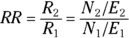
Let’s revisit the example of 2023 incidence of Type II diabetes in adults in City XYZ compared to City ABC. For City XYZ, you have N₁ = 30 and E₁ = 300,000. For City ABC, you have N₁ = 24 and E₂ = 80,000. The RR for City ABC relative to City XYZ is , or 3.0, indicating that City ABC has three times the adult Type II diabetes incidence in 2023 compared to City XYZ. You could calculate the difference between two incidence rates if you wanted to, but in epidemiology, RRs are used much more often than rate differences.

Calculating confidence intervals for a rate ratio

Whenever you report an RR you’ve calculated, you should also indicate how precise it is. The exact calculation of a CI around RR is quite difficult, but if your observed event counts are large enough (meaning ≥ 10), then the following approximate formula for the 95 percent CI around an RR works reasonably well: where .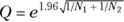

For other confidence levels, you can replace the 1.96 in the Q formula with the appropriate critical z value for the normal distribution.

So, for the 2023 adult Type II diabetes example, you would set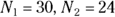, and RR =  3.0. The equation would be 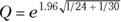, so the 95 percent lower and upper confidence limits would be and , meaning the CI of the RR would be from 1.75 to 5.13. You would interpret this by saying that that 2023 RR for adult Type II diabetes incidence is 3.0 times the rate in City ABC compared to City XYZ (95 percent CI 1.75 to 5.13).

Comparing two event rates

The examples in this chapter have compared incidence (or event) rates of adult Type II diabetes in 2023 between City XYZ and City ABC. These two event rates are represented as for City XYZ, and for City ABC. They are based on City XYZ having an of 30 events and City ABC having an of 24 events, and on exposures and for City XYZ and City ABC, respectively. The difference in event rates between City XYZ and City ABC can be tested for significance by calculating the 95 percent CI around the RR, and observing whether that CI includes the value of 1.0. Because the RR is a ratio, having 1.0 included in the CI indicates that City XYZ’s and City ABC’s rates could be identical. If the 95 percent CI around the RR includes 1, the RR isn’t statistically significantly different from 1, so the two rates aren’t significantly different from each other (assuming α = 0.05). But if the 95 percent CI is either entirely above or entirely below 1.0, the RR is statistically significantly different from 1, so the two rates are significantly different from each other (assuming α = 0.05).

For the City ABC and City XYZ adult Type II diabetes 2023 rate comparison, the observed RR was 3.0, with a 95 percent confidence interval of 1.75 to 5.13. This CI does not include 1.0 — in fact, it is entirely above 1.0. So, the RR is significantly greater than 1, and you would conclude that City ABC has a statistically significantly higher adult Type II diabetes incidence rate than City XYZ (assuming α = 0.05).

Comparing two event counts with identical exposure

If — and only if — the two exposures ( and ) are identical, there’s an extremely simple rule for testing whether two event counts ( and ) are significantly different from each other at the level of α = 0.05: If , then the Ns are statistically significantly different (at α = 0.05).

To interpret the formula into words, if the square of the difference is more than four times the sum, then the event counts are statistically significantly different at α = 0.05. The value of 4 in this rule approximates 3.84, the chi-square value corresponding to p = 0.05.

Imagine you learned that in City XYZ, there were 30 fatal car accidents in 2022. In the following year, 2023, you learned City XYZ had 40 fatal car accidents. You may wonder: Is driving in City XYZ getting more dangerous every year? Or was the observed increase from 2022 to 2023 due to random fluctuations? Using the simple rule, you can calculate , which is less than 4. Having 30 events — which in this case are fatal car accidents — isn’t statistically significantly different from having 40 events in the same time period. As you see from the result, the increase of 10 in one year is likely statistical noise. But had the number of events increased more dramatically — say from 30 to 50 events — the increase would have been statistically significant. This is because , which is greater than 4.